Analysis: Evaluation & Results Analysis
Introduction
Analysis is designed to show the graphical reports of Intraday Trading , which helps users to evaluate and analyse investment portfolios visually. The following are some graphics to view:
- analysis_position
report_graph
score_ic_graph
cumulative_return_graph
risk_analysis_graph
rank_label_graph
- analysis_model
model_performance_graph
All of the accumulated profit metrics(e.g. return, max drawdown) in Qlib are calculated by summation. This avoids the metrics or the plots being skewed exponentially over time.
Graphical Reports
Users can run the following code to get all supported reports.
>> import qlib.contrib.report as qcr
>> print(qcr.GRAPH_NAME_LIST)
['analysis_position.report_graph', 'analysis_position.score_ic_graph', 'analysis_position.cumulative_return_graph', 'analysis_position.risk_analysis_graph', 'analysis_position.rank_label_graph', 'analysis_model.model_performance_graph']
Note
For more details, please refer to the function document: similar to help(qcr.analysis_position.report_graph)
Usage & Example
Usage of analysis_position.report
API
Graphical Result
Note
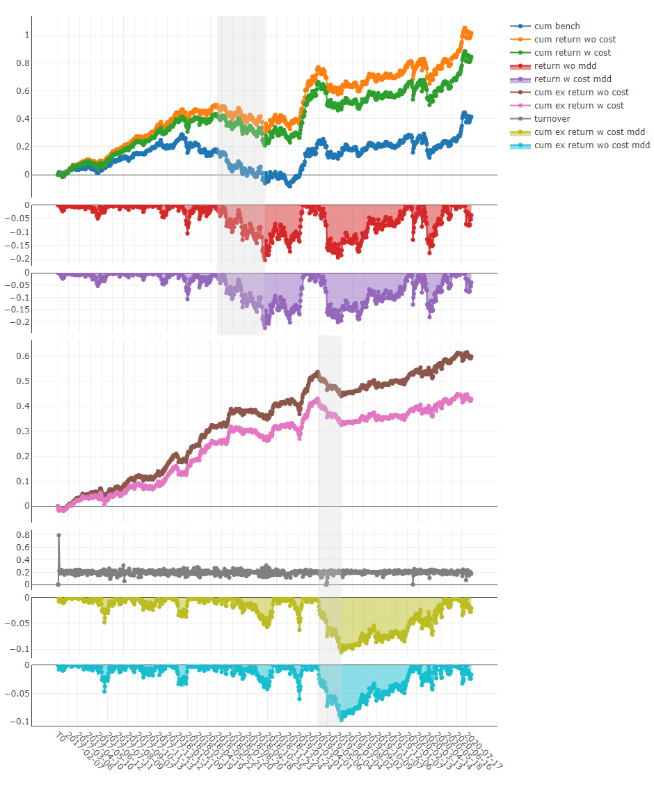
Axis X: Trading day
- Axis Y:
- cum bench
Cumulative returns series of benchmark
- cum return wo cost
Cumulative returns series of portfolio without cost
- cum return w cost
Cumulative returns series of portfolio with cost
- return wo mdd
Maximum drawdown series of cumulative return without cost
- return w cost mdd:
Maximum drawdown series of cumulative return with cost
- cum ex return wo cost
The CAR (cumulative abnormal return) series of the portfolio compared to the benchmark without cost.
- cum ex return w cost
The CAR (cumulative abnormal return) series of the portfolio compared to the benchmark with cost.
- turnover
Turnover rate series
- cum ex return wo cost mdd
Drawdown series of CAR (cumulative abnormal return) without cost
- cum ex return w cost mdd
Drawdown series of CAR (cumulative abnormal return) with cost
The shaded part above: Maximum drawdown corresponding to cum return wo cost
The shaded part below: Maximum drawdown corresponding to cum ex return wo cost
Usage of analysis_position.score_ic
API
Graphical Result
Note
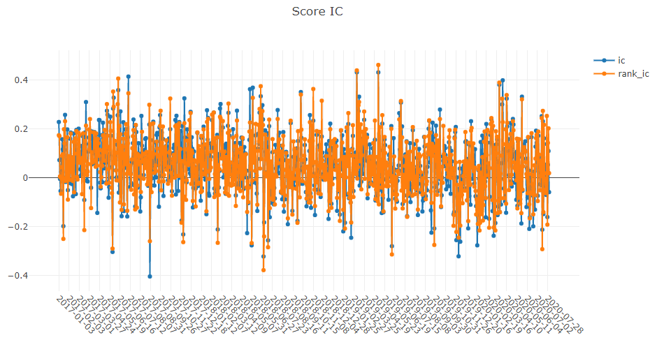
Axis X: Trading day
- Axis Y:
- ic
The Pearson correlation coefficient series between label and prediction score. In the above example, the label is formulated as Ref($close, -2)/Ref($close, -1)-1. Please refer to Data Feature for more details.
- rank_ic
The Spearman’s rank correlation coefficient series between label and prediction score.
Usage of analysis_position.risk_analysis
API
Graphical Result
Note
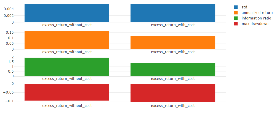
- general graphics
- std
- excess_return_without_cost
The Standard Deviation of CAR (cumulative abnormal return) without cost.
- excess_return_with_cost
The Standard Deviation of CAR (cumulative abnormal return) with cost.
- annualized_return
- excess_return_without_cost
The Annualized Rate of CAR (cumulative abnormal return) without cost.
- excess_return_with_cost
The Annualized Rate of CAR (cumulative abnormal return) with cost.
- information_ratio
- excess_return_without_cost
The Information Ratio without cost.
- excess_return_with_cost
The Information Ratio with cost.
To know more about Information Ratio, please refer to Information Ratio – IR.
- max_drawdown
- excess_return_without_cost
The Maximum Drawdown of CAR (cumulative abnormal return) without cost.
- excess_return_with_cost
The Maximum Drawdown of CAR (cumulative abnormal return) with cost.
Note
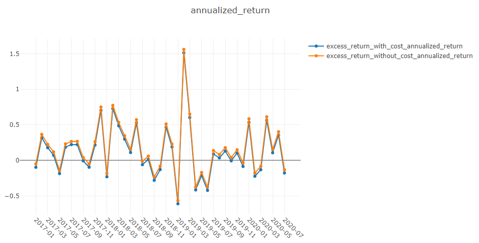
- annualized_return/max_drawdown/information_ratio/std graphics
Axis X: Trading days grouped by month
- Axis Y:
- annualized_return graphics
- excess_return_without_cost_annualized_return
The Annualized Rate series of monthly CAR (cumulative abnormal return) without cost.
- excess_return_with_cost_annualized_return
The Annualized Rate series of monthly CAR (cumulative abnormal return) with cost.
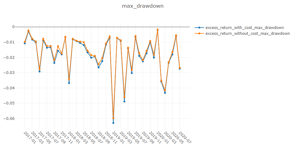
- max_drawdown graphics
- excess_return_without_cost_max_drawdown
The Maximum Drawdown series of monthly CAR (cumulative abnormal return) without cost.
- excess_return_with_cost_max_drawdown
The Maximum Drawdown series of monthly CAR (cumulative abnormal return) with cost.
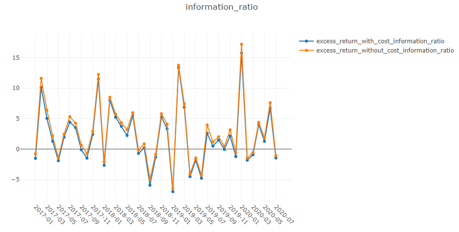
- information_ratio graphics
- excess_return_without_cost_information_ratio
The Information Ratio series of monthly CAR (cumulative abnormal return) without cost.
- excess_return_with_cost_information_ratio
The Information Ratio series of monthly CAR (cumulative abnormal return) with cost.
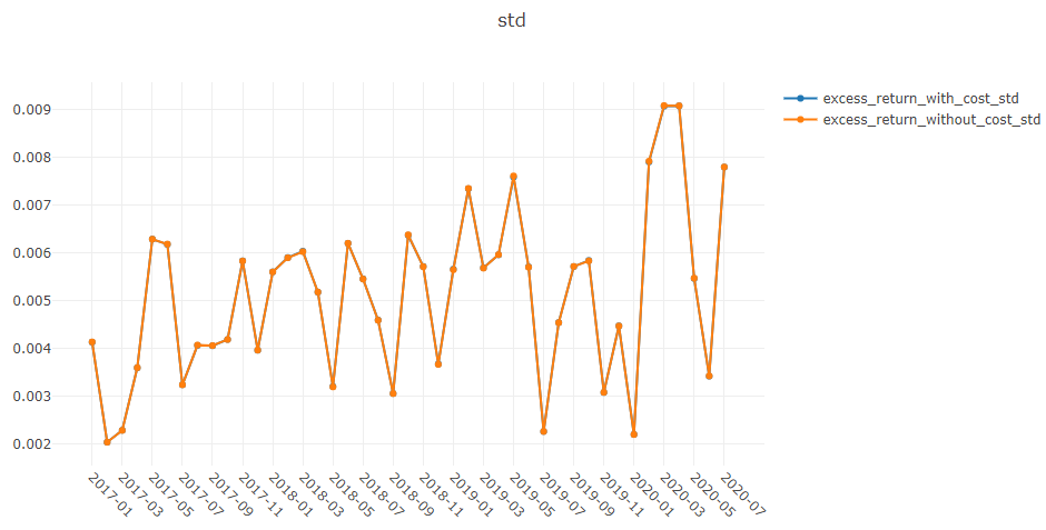
- std graphics
- excess_return_without_cost_max_drawdown
The Standard Deviation series of monthly CAR (cumulative abnormal return) without cost.
- excess_return_with_cost_max_drawdown
The Standard Deviation series of monthly CAR (cumulative abnormal return) with cost.
Usage of analysis_model.analysis_model_performance
API
Graphical Results
Note
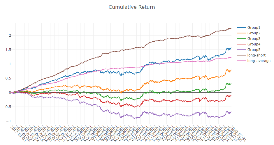
- cumulative return graphics
- Group1:
The Cumulative Return series of stocks group with (ranking ratio of label <= 20%)
- Group2:
The Cumulative Return series of stocks group with (20% < ranking ratio of label <= 40%)
- Group3:
The Cumulative Return series of stocks group with (40% < ranking ratio of label <= 60%)
- Group4:
The Cumulative Return series of stocks group with (60% < ranking ratio of label <= 80%)
- Group5:
The Cumulative Return series of stocks group with (80% < ranking ratio of label)
- long-short:
The Difference series between Cumulative Return of Group1 and of Group5
- long-average
The Difference series between Cumulative Return of Group1 and average Cumulative Return for all stocks.
- The ranking ratio can be formulated as follows.
- \[ranking\ ratio = \frac{Ascending\ Ranking\ of\ label}{Number\ of\ Stocks\ in\ the\ Portfolio}\]
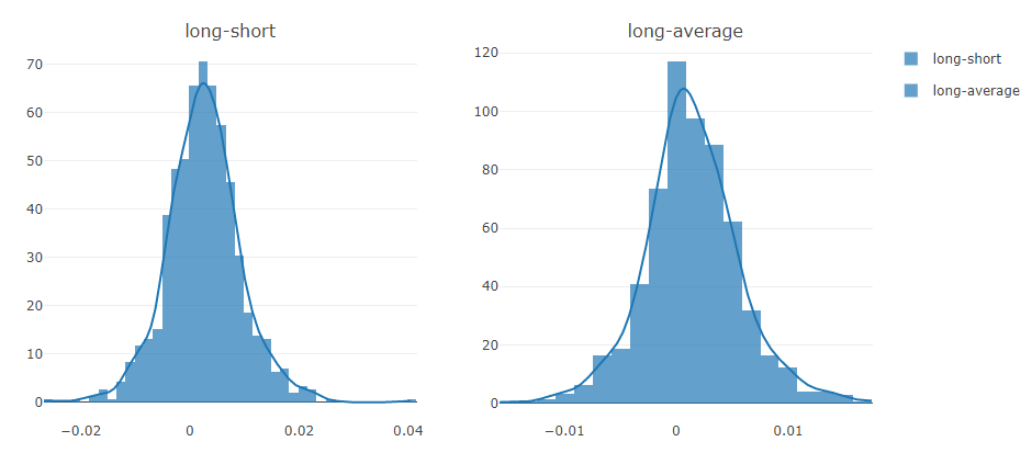
Note
- long-short/long-average
The distribution of long-short/long-average returns on each trading day
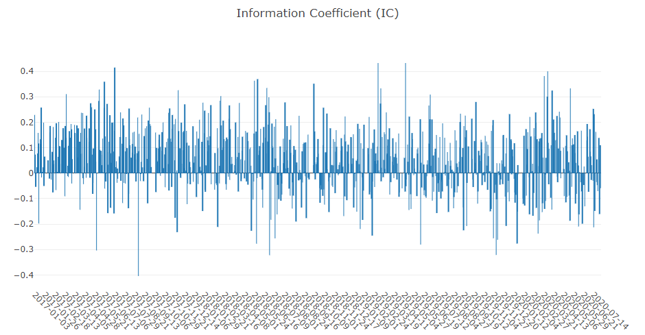
Note
- Information Coefficient
The Pearson correlation coefficient series between labels and prediction scores of stocks in portfolio.
The graphics reports can be used to evaluate the prediction scores.
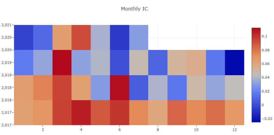
Note
- Monthly IC
Monthly average of the Information Coefficient
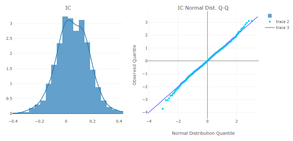
Note
- IC
The distribution of the Information Coefficient on each trading day.
- IC Normal Dist. Q-Q
The Quantile-Quantile Plot is used for the normal distribution of Information Coefficient on each trading day.
Note
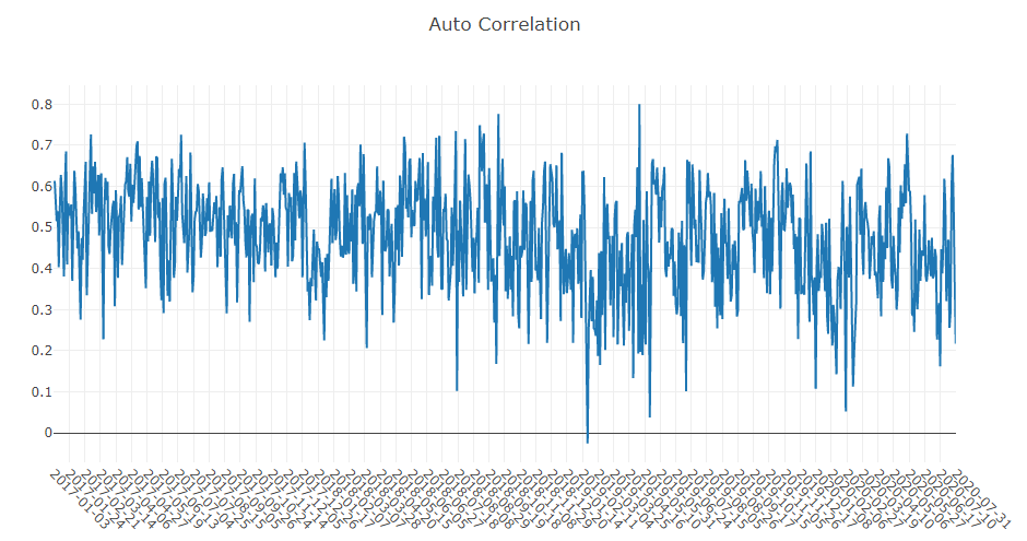
- Auto Correlation
The Pearson correlation coefficient series between the latest prediction scores and the prediction scores lag days ago of stocks in portfolio on each trading day.
The graphics reports can be used to estimate the turnover rate.