Portfolio Strategy: Portfolio Management
Introduction
Portfolio Strategy is designed to adopt different portfolio strategies, which means that users can adopt different algorithms to generate investment portfolios based on the prediction scores of the Forecast Model. Users can use the Portfolio Strategy in an automatic workflow by Workflow module, please refer to Workflow: Workflow Management.
Because the components in Qlib are designed in a loosely-coupled way, Portfolio Strategy can be used as an independent module also.
Qlib provides several implemented portfolio strategies. Also, Qlib supports custom strategy, users can customize strategies according to their own requirements.
After users specifying the models(forecasting signals) and strategies, running backtest will help users to check the performance of a custom model(forecasting signals)/strategy.
Base Class & Interface
BaseStrategy
Qlib provides a base class qlib.strategy.base.BaseStrategy. All strategy classes need to inherit the base class and implement its interface.
- get_risk_degree
- Return the proportion of your total value you will use in investment. Dynamically risk_degree will result in Market timing.
- generate_order_list
- Return the order list. The frequency to call this method depends on the executor frequency(“time_per_step”=”day” by default). But the trading frequency can be decided by users’ implementation. For example, if the user wants to trading in weekly while the time_per_step is “day” in executor, user can return non-empty TradeDecision weekly(otherwise return empty like this ).
Users can inherit BaseStrategy to customize their strategy class.
WeightStrategyBase
Qlib also provides a class qlib.contrib.strategy.WeightStrategyBase that is a subclass of BaseStrategy.
WeightStrategyBase only focuses on the target positions, and automatically generates an order list based on positions. It provides the generate_target_weight_position interface.
- generate_target_weight_position
- According to the current position and trading date to generate the target position. The cash is not considered in the output weight distribution.
- Return the target position.
Note
Here the target position means the target percentage of total assets.
WeightStrategyBase implements the interface generate_order_list, whose processions is as follows.
- Call generate_target_weight_position method to generate the target position.
- Generate the target amount of stocks from the target position.
- Generate the order list from the target amount
Users can inherit WeightStrategyBase and implement the interface generate_target_weight_position to customize their strategy class, which only focuses on the target positions.
Implemented Strategy
Qlib provides a implemented strategy classes named TopkDropoutStrategy.
TopkDropoutStrategy
TopkDropoutStrategy is a subclass of BaseStrategy and implement the interface generate_order_list whose process is as follows.
Adopt the
Topk-Dropalgorithm to calculate the target amount of each stockNote
Topk-Dropalgorithm:- Topk: The number of stocks held
- Drop: The number of stocks sold on each trading day
Currently, the number of held stocks is Topk. On each trading day, the Drop number of held stocks with the worst prediction score will be sold, and the same number of unheld stocks with the best prediction score will be bought.
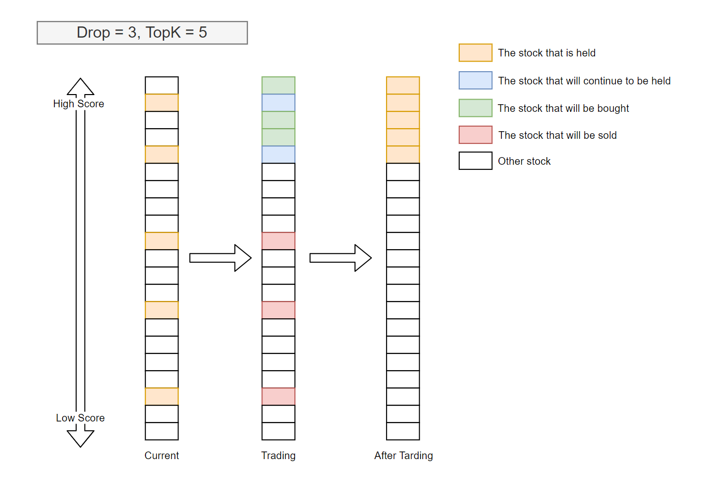
TopkDropalgorithm sells Drop stocks every trading day, which guarantees a fixed turnover rate.Generate the order list from the target amount
EnhancedIndexingStrategy
EnhancedIndexingStrategy Enhanced indexing combines the arts of active management and passive management, with the aim of outperforming a benchmark index (e.g., S&P 500) in terms of portfolio return while controlling the risk exposure (a.k.a. tracking error).
For more information, please refer to qlib.contrib.strategy.signal_strategy.EnhancedIndexingStrategy and qlib.contrib.strategy.optimizer.enhanced_indexing.EnhancedIndexingOptimizer.
Usage & Example
First, user can create a model to get trading signals(the variable name is pred_score in following cases).
Prediction Score
The prediction score is a pandas DataFrame. Its index is <datetime(pd.Timestamp), instrument(str)> and it must contains a score column.
A prediction sample is shown as follows.
  datetime instrument     score
2019-01-04   SH600000 -0.505488
2019-01-04   SZ002531 -0.320391
2019-01-04   SZ000999  0.583808
2019-01-04   SZ300569  0.819628
2019-01-04   SZ001696 -0.137140
             ...            ...
2019-04-30   SZ000996 -1.027618
2019-04-30   SH603127  0.225677
2019-04-30   SH603126  0.462443
2019-04-30   SH603133 -0.302460
2019-04-30   SZ300760 -0.126383
Forecast Model module can make predictions, please refer to Forecast Model: Model Training & Prediction.
Normally, the prediction score is the output of the models. But some models are learned from a label with a different scale. So the scale of the prediction score may be different from your expectation(e.g. the return of instruments).
Qlib didn’t add a step to scale the prediction score to a unified scale. Because not every trading strategy cares about the scale(e.g. TopkDropoutStrategy only cares about the order). So the strategy is responsible for rescaling the prediction score(e.g. some portfolio-optimization-based strategies may require a meaningful scale).
Running backtest
In most cases, users could backtest their portfolio management strategy with
backtest_daily.from pprint import pprint import qlib import pandas as pd from qlib.utils.time import Freq from qlib.utils import flatten_dict from qlib.contrib.evaluate import backtest_daily from qlib.contrib.evaluate import risk_analysis from qlib.contrib.strategy import TopkDropoutStrategy # init qlib qlib.init(provider_uri=<qlib data dir>) CSI300_BENCH = "SH000300" STRATEGY_CONFIG = { "topk": 50, "n_drop": 5, # pred_score, pd.Series "signal": pred_score, } strategy_obj = TopkDropoutStrategy(**STRATEGY_CONFIG) report_normal, positions_normal = backtest_daily( start_time="2017-01-01", end_time="2020-08-01", strategy=strategy_obj ) analysis = dict() analysis["excess_return_without_cost"] = risk_analysis( report_normal["return"] - report_normal["bench"], freq=analysis_freq ) analysis["excess_return_with_cost"] = risk_analysis( report_normal["return"] - report_normal["bench"] - report_normal["cost"], freq=analysis_freq ) analysis_df = pd.concat(analysis) # type: pd.DataFrame pprint(analysis_df)
If users would like to control their strategies in a more detailed(e.g. users have a more advanced version of executor), user could follow this example.
from pprint import pprint

import qlib
import pandas as pd
from qlib.utils.time import Freq
from qlib.utils import flatten_dict
from qlib.backtest import backtest, executor
from qlib.contrib.evaluate import risk_analysis
from qlib.contrib.strategy import TopkDropoutStrategy

# init qlib
qlib.init(provider_uri=<qlib data dir>)

CSI300_BENCH = "SH000300"
FREQ = "day"
STRATEGY_CONFIG = {
    "topk": 50,
    "n_drop": 5,
    # pred_score, pd.Series
    "signal": pred_score,
}

EXECUTOR_CONFIG = {
    "time_per_step": "day",
    "generate_portfolio_metrics": True,
}

backtest_config = {
    "start_time": "2017-01-01",
    "end_time": "2020-08-01",
    "account": 100000000,
    "benchmark": CSI300_BENCH,
    "exchange_kwargs": {
        "freq": FREQ,
        "limit_threshold": 0.095,
        "deal_price": "close",
        "open_cost": 0.0005,
        "close_cost": 0.0015,
        "min_cost": 5,
    },
}

# strategy object
strategy_obj = TopkDropoutStrategy(**STRATEGY_CONFIG)
# executor object
executor_obj = executor.SimulatorExecutor(**EXECUTOR_CONFIG)
# backtest
portfolio_metric_dict, indicator_dict = backtest(executor=executor_obj, strategy=strategy_obj, **backtest_config)
analysis_freq = "{0}{1}".format(*Freq.parse(FREQ))
# backtest info
report_normal, positions_normal = portfolio_metric_dict.get(analysis_freq)

# analysis
analysis = dict()
analysis["excess_return_without_cost"] = risk_analysis(
    report_normal["return"] - report_normal["bench"], freq=analysis_freq
)
analysis["excess_return_with_cost"] = risk_analysis(
    report_normal["return"] - report_normal["bench"] - report_normal["cost"], freq=analysis_freq
)

analysis_df = pd.concat(analysis)  # type: pd.DataFrame
# log metrics
analysis_dict = flatten_dict(analysis_df["risk"].unstack().T.to_dict())
# print out results
pprint(f"The following are analysis results of benchmark return({analysis_freq}).")
pprint(risk_analysis(report_normal["bench"], freq=analysis_freq))
pprint(f"The following are analysis results of the excess return without cost({analysis_freq}).")
pprint(analysis["excess_return_without_cost"])
pprint(f"The following are analysis results of the excess return with cost({analysis_freq}).")
pprint(analysis["excess_return_with_cost"])
Result
The backtest results are in the following form:
                                                  risk
excess_return_without_cost mean               0.000605
                           std                0.005481
                           annualized_return  0.152373
                           information_ratio  1.751319
                           max_drawdown      -0.059055
excess_return_with_cost    mean               0.000410
                           std                0.005478
                           annualized_return  0.103265
                           information_ratio  1.187411
                           max_drawdown      -0.075024
- excess_return_without_cost
- mean
- Mean value of the CAR (cumulative abnormal return) without cost
- std
- The Standard Deviation of CAR (cumulative abnormal return) without cost.
- annualized_return
- The Annualized Rate of CAR (cumulative abnormal return) without cost.
- information_ratio
- The Information Ratio without cost. please refer to Information Ratio – IR.
- max_drawdown
- The Maximum Drawdown of CAR (cumulative abnormal return) without cost, please refer to Maximum Drawdown (MDD).
- excess_return_with_cost
- mean
- Mean value of the CAR (cumulative abnormal return) series with cost
- std
- The Standard Deviation of CAR (cumulative abnormal return) series with cost.
- annualized_return
- The Annualized Rate of CAR (cumulative abnormal return) with cost.
- information_ratio
- The Information Ratio with cost. please refer to Information Ratio – IR.
- max_drawdown
- The Maximum Drawdown of CAR (cumulative abnormal return) with cost, please refer to Maximum Drawdown (MDD).
Reference
To know more about the prediction score pred_score output by Forecast Model, please refer to Forecast Model: Model Training & Prediction.