Analysis: Evaluation & Results Analysis
Introduction
Analysis is designed to show the graphical reports of Intraday Trading , which helps users to evaluate and analyse investment portfolios visually. The following are some graphics to view:
- analysis_position
- report_graph
- score_ic_graph
- cumulative_return_graph
- risk_analysis_graph
- rank_label_graph
- analysis_model
- model_performance_graph
All of the accumulated profit metrics(e.g. return, max drawdown) in Qlib are calculated by summation. This avoids the metrics or the plots being skewed exponentially over time.
Graphical Reports
Users can run the following code to get all supported reports.
>> import qlib.contrib.report as qcr
>> print(qcr.GRAPH_NAME_LIST)
['analysis_position.report_graph', 'analysis_position.score_ic_graph', 'analysis_position.cumulative_return_graph', 'analysis_position.risk_analysis_graph', 'analysis_position.rank_label_graph', 'analysis_model.model_performance_graph']
Note
For more details, please refer to the function document: similar to help(qcr.analysis_position.report_graph)
Usage & Example
Usage of analysis_position.report
API
-
qlib.contrib.report.analysis_position.report.report_graph(report_df: pandas.core.frame.DataFrame, show_notebook: bool = True) → [<class 'list'>, <class 'tuple'>] display backtest report
Example:
import qlib
import pandas as pd
from qlib.utils.time import Freq
from qlib.utils import flatten_dict
from qlib.backtest import backtest, executor
from qlib.contrib.evaluate import risk_analysis
from qlib.contrib.strategy import TopkDropoutStrategy

# init qlib
qlib.init(provider_uri=<qlib data dir>)

CSI300_BENCH = "SH000300"
FREQ = "day"
STRATEGY_CONFIG = {
    "topk": 50,
    "n_drop": 5,
    # pred_score, pd.Series
    "signal": pred_score,
}

EXECUTOR_CONFIG = {
    "time_per_step": "day",
    "generate_portfolio_metrics": True,
}

backtest_config = {
    "start_time": "2017-01-01",
    "end_time": "2020-08-01",
    "account": 100000000,
    "benchmark": CSI300_BENCH,
    "exchange_kwargs": {
        "freq": FREQ,
        "limit_threshold": 0.095,
        "deal_price": "close",
        "open_cost": 0.0005,
        "close_cost": 0.0015,
        "min_cost": 5,
    },
}

# strategy object
strategy_obj = TopkDropoutStrategy(**STRATEGY_CONFIG)
# executor object
executor_obj = executor.SimulatorExecutor(**EXECUTOR_CONFIG)
# backtest
portfolio_metric_dict, indicator_dict = backtest(executor=executor_obj, strategy=strategy_obj, **backtest_config)
analysis_freq = "{0}{1}".format(*Freq.parse(FREQ))
# backtest info
report_normal_df, positions_normal = portfolio_metric_dict.get(analysis_freq)

qcr.analysis_position.report_graph(report_normal_df)
Parameters: - report_df –
df.index.name must be date, df.columns must contain return, turnover, cost, bench.
            return      cost        bench       turnover
date
2017-01-04  0.003421    0.000864    0.011693    0.576325
2017-01-05  0.000508    0.000447    0.000721    0.227882
2017-01-06  -0.003321   0.000212    -0.004322   0.102765
2017-01-09  0.006753    0.000212    0.006874    0.105864
2017-01-10  -0.000416   0.000440    -0.003350   0.208396
- show_notebook – whether to display graphics in notebook, the default is True.
Returns: if show_notebook is True, display in notebook; else return plotly.graph_objs.Figure list.
- report_df –
Graphical Result
Note
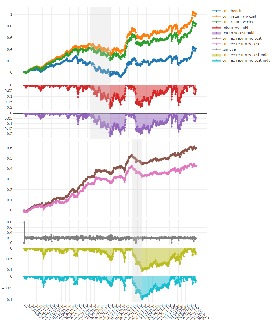
- Axis X: Trading day
- Axis Y:
- cum bench
- Cumulative returns series of benchmark
- cum return wo cost
- Cumulative returns series of portfolio without cost
- cum return w cost
- Cumulative returns series of portfolio with cost
- return wo mdd
- Maximum drawdown series of cumulative return without cost
- return w cost mdd:
- Maximum drawdown series of cumulative return with cost
- cum ex return wo cost
- The CAR (cumulative abnormal return) series of the portfolio compared to the benchmark without cost.
- cum ex return w cost
- The CAR (cumulative abnormal return) series of the portfolio compared to the benchmark with cost.
- turnover
- Turnover rate series
- cum ex return wo cost mdd
- Drawdown series of CAR (cumulative abnormal return) without cost
- cum ex return w cost mdd
- Drawdown series of CAR (cumulative abnormal return) with cost
- The shaded part above: Maximum drawdown corresponding to cum return wo cost
- The shaded part below: Maximum drawdown corresponding to cum ex return wo cost
Usage of analysis_position.score_ic
API
-
qlib.contrib.report.analysis_position.score_ic.score_ic_graph(pred_label: pandas.core.frame.DataFrame, show_notebook: bool = True) → [<class 'list'>, <class 'tuple'>] score IC
Example:
from qlib.data import D
from qlib.contrib.report import analysis_position
pred_df_dates = pred_df.index.get_level_values(level='datetime')
features_df = D.features(D.instruments('csi500'), ['Ref($close, -2)/Ref($close, -1)-1'], pred_df_dates.min(), pred_df_dates.max())
features_df.columns = ['label']
pred_label = pd.concat([features_df, pred], axis=1, sort=True).reindex(features_df.index)
analysis_position.score_ic_graph(pred_label)
Parameters: - pred_label –
index is pd.MultiIndex, index name is [instrument, datetime]; columns names is [score, label].
instrument  datetime        score         label
SH600004  2017-12-11     -0.013502       -0.013502
            2017-12-12   -0.072367       -0.072367
            2017-12-13   -0.068605       -0.068605
            2017-12-14    0.012440        0.012440
            2017-12-15   -0.102778       -0.102778
- show_notebook – whether to display graphics in notebook, the default is True.
Returns: if show_notebook is True, display in notebook; else return plotly.graph_objs.Figure list.
- pred_label –
Graphical Result
Note
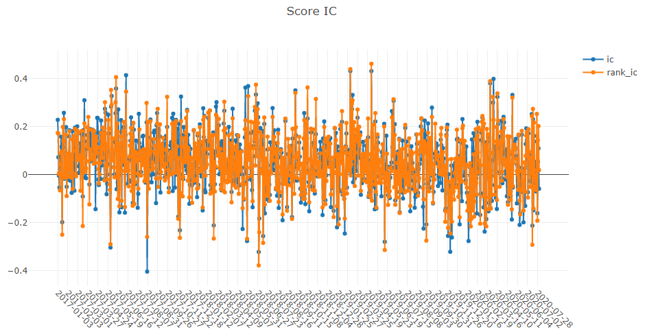
- Axis X: Trading day
- Axis Y:
- ic
- The Pearson correlation coefficient series between label and prediction score. In the above example, the label is formulated as Ref($close, -2)/Ref($close, -1)-1. Please refer to Data Feature for more details.
- rank_ic
- The Spearman’s rank correlation coefficient series between label and prediction score.
Usage of analysis_position.risk_analysis
API
-
qlib.contrib.report.analysis_position.risk_analysis.risk_analysis_graph(analysis_df: pandas.core.frame.DataFrame = None, report_normal_df: pandas.core.frame.DataFrame = None, report_long_short_df: pandas.core.frame.DataFrame = None, show_notebook: bool = True) → Iterable[plotly.graph_objs._figure.Figure] Generate analysis graph and monthly analysis
Example:
import qlib
import pandas as pd
from qlib.utils.time import Freq
from qlib.utils import flatten_dict
from qlib.backtest import backtest, executor
from qlib.contrib.evaluate import risk_analysis
from qlib.contrib.strategy import TopkDropoutStrategy

# init qlib
qlib.init(provider_uri=<qlib data dir>)

CSI300_BENCH = "SH000300"
FREQ = "day"
STRATEGY_CONFIG = {
    "topk": 50,
    "n_drop": 5,
    # pred_score, pd.Series
    "signal": pred_score,
}

EXECUTOR_CONFIG = {
    "time_per_step": "day",
    "generate_portfolio_metrics": True,
}

backtest_config = {
    "start_time": "2017-01-01",
    "end_time": "2020-08-01",
    "account": 100000000,
    "benchmark": CSI300_BENCH,
    "exchange_kwargs": {
        "freq": FREQ,
        "limit_threshold": 0.095,
        "deal_price": "close",
        "open_cost": 0.0005,
        "close_cost": 0.0015,
        "min_cost": 5,
    },
}

# strategy object
strategy_obj = TopkDropoutStrategy(**STRATEGY_CONFIG)
# executor object
executor_obj = executor.SimulatorExecutor(**EXECUTOR_CONFIG)
# backtest
portfolio_metric_dict, indicator_dict = backtest(executor=executor_obj, strategy=strategy_obj, **backtest_config)
analysis_freq = "{0}{1}".format(*Freq.parse(FREQ))
# backtest info
report_normal_df, positions_normal = portfolio_metric_dict.get(analysis_freq)
analysis = dict()
analysis["excess_return_without_cost"] = risk_analysis(
    report_normal_df["return"] - report_normal_df["bench"], freq=analysis_freq
)
analysis["excess_return_with_cost"] = risk_analysis(
    report_normal_df["return"] - report_normal_df["bench"] - report_normal_df["cost"], freq=analysis_freq
)

analysis_df = pd.concat(analysis)  # type: pd.DataFrame
analysis_position.risk_analysis_graph(analysis_df, report_normal_df)
Parameters: - analysis_df –
analysis data, index is pd.MultiIndex; columns names is [risk].
                                                  risk
excess_return_without_cost mean               0.000692
                           std                0.005374
                           annualized_return  0.174495
                           information_ratio  2.045576
                           max_drawdown      -0.079103
excess_return_with_cost    mean               0.000499
                           std                0.005372
                           annualized_return  0.125625
                           information_ratio  1.473152
                           max_drawdown      -0.088263
- report_normal_df –
df.index.name must be date, df.columns must contain return, turnover, cost, bench.
            return      cost        bench       turnover
date
2017-01-04  0.003421    0.000864    0.011693    0.576325
2017-01-05  0.000508    0.000447    0.000721    0.227882
2017-01-06  -0.003321   0.000212    -0.004322   0.102765
2017-01-09  0.006753    0.000212    0.006874    0.105864
2017-01-10  -0.000416   0.000440    -0.003350   0.208396
- report_long_short_df –
df.index.name must be date, df.columns contain long, short, long_short.
            long        short       long_short
date
2017-01-04  -0.001360   0.001394    0.000034
2017-01-05  0.002456    0.000058    0.002514
2017-01-06  0.000120    0.002739    0.002859
2017-01-09  0.001436    0.001838    0.003273
2017-01-10  0.000824    -0.001944   -0.001120
- show_notebook – Whether to display graphics in a notebook, default True. If True, show graph in notebook If False, return graph figure
Returns: - analysis_df –
Graphical Result
Note
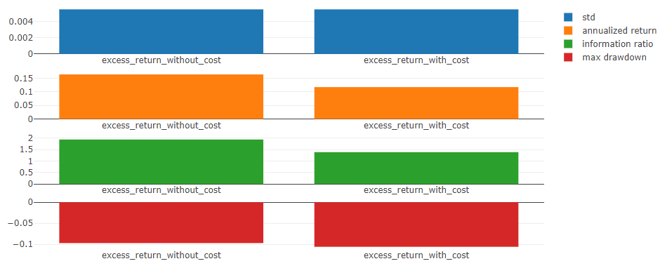
- general graphics
- std
- excess_return_without_cost
- The Standard Deviation of CAR (cumulative abnormal return) without cost.
- excess_return_with_cost
- The Standard Deviation of CAR (cumulative abnormal return) with cost.
- annualized_return
- excess_return_without_cost
- The Annualized Rate of CAR (cumulative abnormal return) without cost.
- excess_return_with_cost
- The Annualized Rate of CAR (cumulative abnormal return) with cost.
- information_ratio
- excess_return_without_cost
- The Information Ratio without cost.
- excess_return_with_cost
- The Information Ratio with cost.
To know more about Information Ratio, please refer to Information Ratio – IR.
- max_drawdown
- excess_return_without_cost
- The Maximum Drawdown of CAR (cumulative abnormal return) without cost.
- excess_return_with_cost
- The Maximum Drawdown of CAR (cumulative abnormal return) with cost.
Note
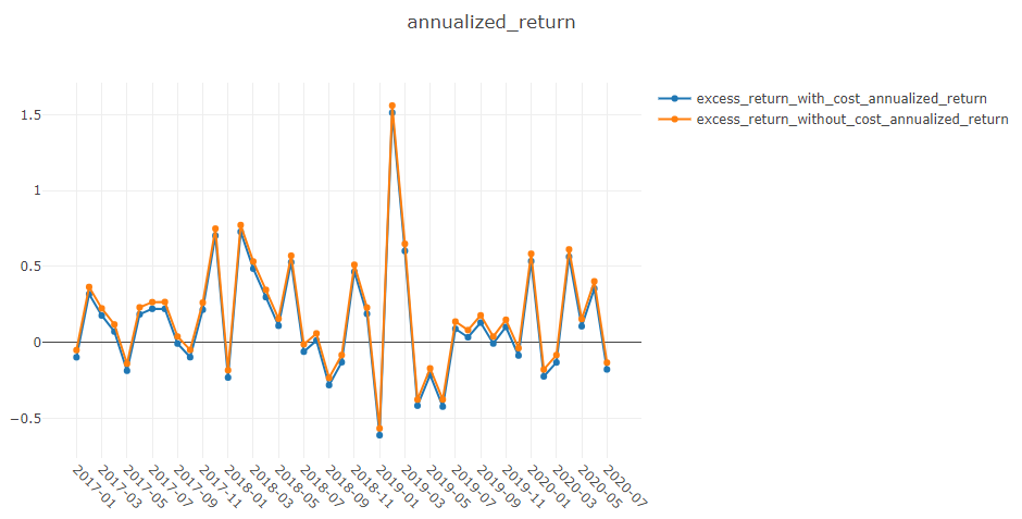
- annualized_return/max_drawdown/information_ratio/std graphics
- Axis X: Trading days grouped by month
- Axis Y:
- annualized_return graphics
- excess_return_without_cost_annualized_return
- The Annualized Rate series of monthly CAR (cumulative abnormal return) without cost.
- excess_return_with_cost_annualized_return
- The Annualized Rate series of monthly CAR (cumulative abnormal return) with cost.
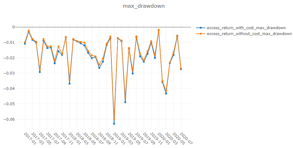
- max_drawdown graphics
- excess_return_without_cost_max_drawdown
- The Maximum Drawdown series of monthly CAR (cumulative abnormal return) without cost.
- excess_return_with_cost_max_drawdown
- The Maximum Drawdown series of monthly CAR (cumulative abnormal return) with cost.
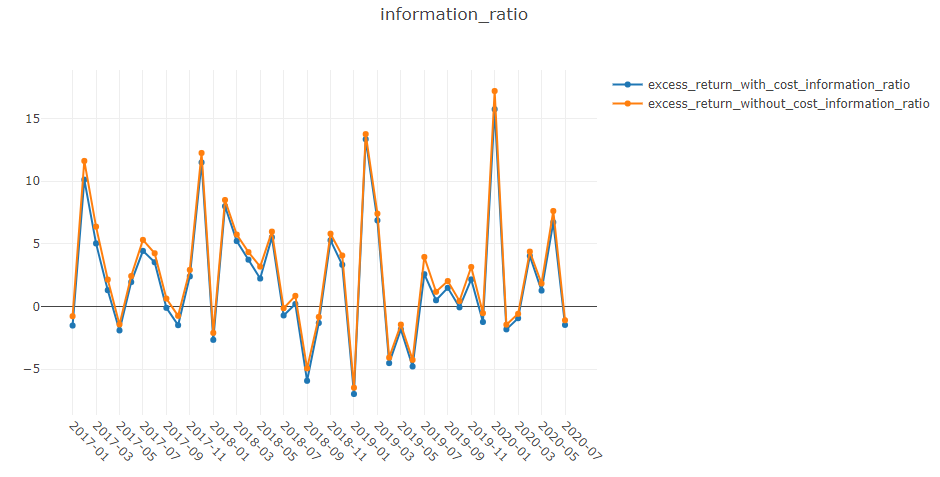
- information_ratio graphics
- excess_return_without_cost_information_ratio
- The Information Ratio series of monthly CAR (cumulative abnormal return) without cost.
- excess_return_with_cost_information_ratio
- The Information Ratio series of monthly CAR (cumulative abnormal return) with cost.
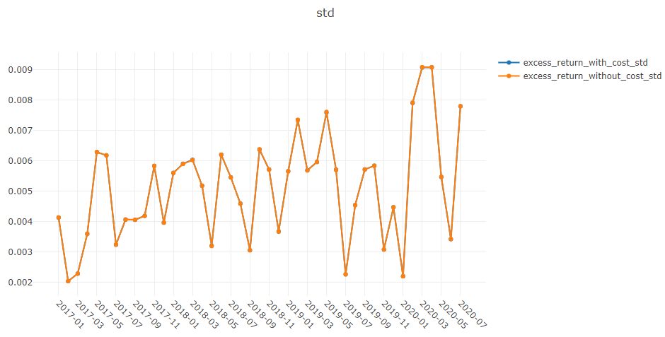
- std graphics
- excess_return_without_cost_max_drawdown
- The Standard Deviation series of monthly CAR (cumulative abnormal return) without cost.
- excess_return_with_cost_max_drawdown
- The Standard Deviation series of monthly CAR (cumulative abnormal return) with cost.
Usage of analysis_model.analysis_model_performance
API
-
qlib.contrib.report.analysis_model.analysis_model_performance.ic_figure(ic_df: pandas.core.frame.DataFrame, show_nature_day=True, **kwargs) → plotly.graph_objs._figure.Figure IC figure
Parameters: - ic_df – ic DataFrame
- show_nature_day – whether to display the abscissa of non-trading day
Returns: plotly.graph_objs.Figure
-
qlib.contrib.report.analysis_model.analysis_model_performance.model_performance_graph(pred_label: pandas.core.frame.DataFrame, lag: int = 1, N: int = 5, reverse=False, rank=False, graph_names: list = ['group_return', 'pred_ic', 'pred_autocorr'], show_notebook: bool = True, show_nature_day=True) → [<class 'list'>, <class 'tuple'>] Model performance
Parameters: - pred_label –
index is pd.MultiIndex, index name is [instrument, datetime]; columns names is [score, label]. It is usually same as the label of model training(e.g. “Ref($close, -2)/Ref($close, -1) - 1”).
instrument  datetime        score       label
SH600004    2017-12-11  -0.013502       -0.013502
                2017-12-12  -0.072367       -0.072367
                2017-12-13  -0.068605       -0.068605
                2017-12-14  0.012440        0.012440
                2017-12-15  -0.102778       -0.102778
- lag – pred.groupby(level=’instrument’)[‘score’].shift(lag). It will be only used in the auto-correlation computing.
- N – group number, default 5.
- reverse – if True, pred[‘score’] *= -1.
- rank – if True, calculate rank ic.
- graph_names – graph names; default [‘cumulative_return’, ‘pred_ic’, ‘pred_autocorr’, ‘pred_turnover’].
- show_notebook – whether to display graphics in notebook, the default is True.
- show_nature_day – whether to display the abscissa of non-trading day.
Returns: if show_notebook is True, display in notebook; else return plotly.graph_objs.Figure list.
- pred_label –
Graphical Results
Note
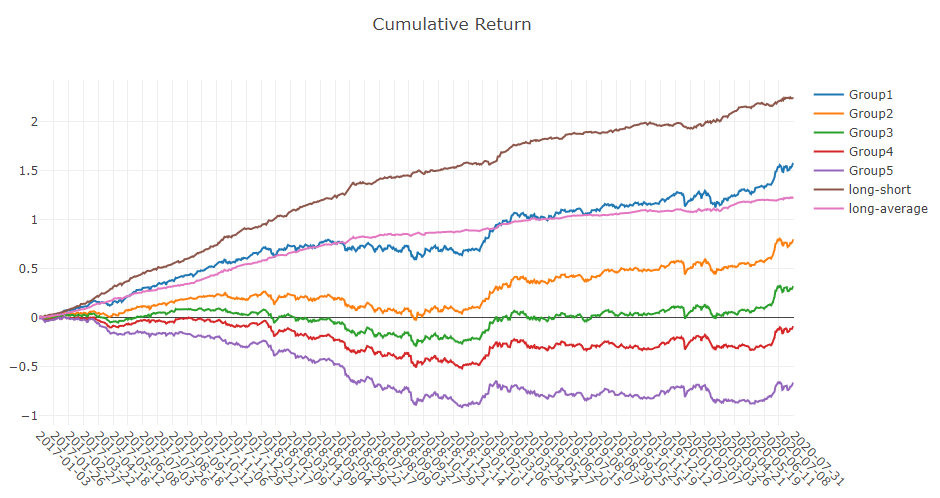
- cumulative return graphics
- Group1:
- The Cumulative Return series of stocks group with (ranking ratio of label <= 20%)
- Group2:
- The Cumulative Return series of stocks group with (20% < ranking ratio of label <= 40%)
- Group3:
- The Cumulative Return series of stocks group with (40% < ranking ratio of label <= 60%)
- Group4:
- The Cumulative Return series of stocks group with (60% < ranking ratio of label <= 80%)
- Group5:
- The Cumulative Return series of stocks group with (80% < ranking ratio of label)
- long-short:
- The Difference series between Cumulative Return of Group1 and of Group5
- long-average
- The Difference series between Cumulative Return of Group1 and average Cumulative Return for all stocks.
- The ranking ratio can be formulated as follows.
- \[ranking\ ratio = \frac{Ascending\ Ranking\ of\ label}{Number\ of\ Stocks\ in\ the\ Portfolio}\]
Note
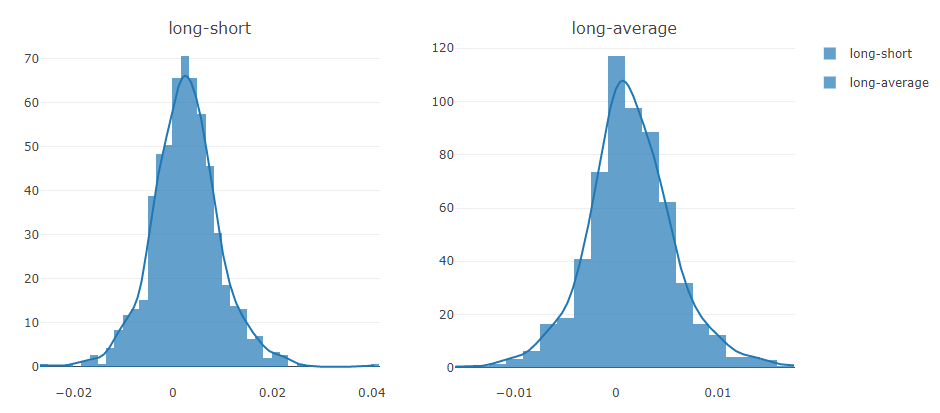
- long-short/long-average
- The distribution of long-short/long-average returns on each trading day
Note
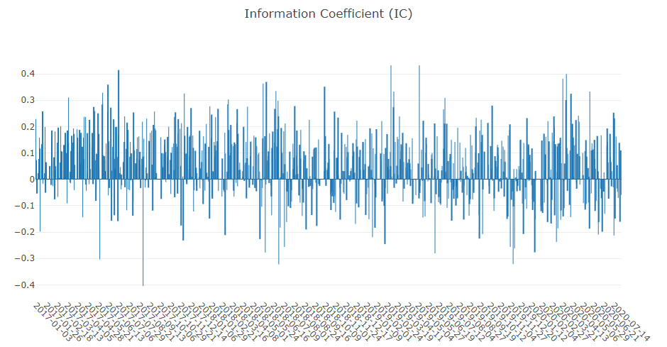
- Information Coefficient
- The Pearson correlation coefficient series between labels and prediction scores of stocks in portfolio.
- The graphics reports can be used to evaluate the prediction scores.
Note
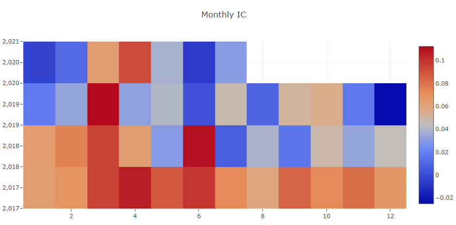
- Monthly IC
- Monthly average of the Information Coefficient
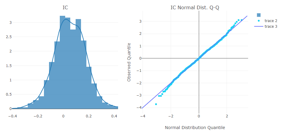
Note
- IC
- The distribution of the Information Coefficient on each trading day.
- IC Normal Dist. Q-Q
- The Quantile-Quantile Plot is used for the normal distribution of Information Coefficient on each trading day.
Note
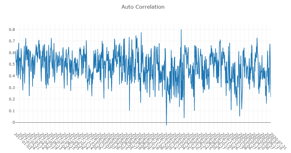
- Auto Correlation
- The Pearson correlation coefficient series between the latest prediction scores and the prediction scores lag days ago of stocks in portfolio on each trading day.
- The graphics reports can be used to estimate the turnover rate.